Interactive companion — This proof has two interactive companions. They render the sphere and the disk side by side as the same cosmos in different coordinates: The Witness Disk (flat-earth view from above) · The Three Witnesses (sphere view).
Introduction
One of the longest-running debates in cosmology pits two pictures of the Earth against each other: a sphere viewed from the outside, or a flat disk with celestial bodies in their circuits above it. The argument usually proceeds as if these were rival empirical claims, each with its own evidence to be weighed.
That framing is too crude. There are not only two empirical claims here. There are at least two distinct philosophical and mathematical claims bundled under the label flat earth, and they must be separated before the discussion can become clear.
Claim A: The flat-disk representation is a coordinate description of the same underlying spherical geometry. The “ice ring” is the South Pole represented as the boundary of an azimuthal disk. The “circuits” of celestial bodies are the same celestial motions expressed in a different coordinate vocabulary. In this sense, the disk and the sphere are not two competing geometries. They are one geometry written in two coordinate systems.
Claim B: The flat-disk representation describes a geometrically distinct reality. On this claim, the ordinary Euclidean flat metric — distances measured with a ruler on the page — is the true metric of Earth’s surface. The sphere is wrong not merely as a vocabulary, but as the underlying geometry.
The purpose of this post is to prove Claim A carefully. A sphere can be represented as a disk by azimuthal projection, and if the disk is equipped with the pulled-back spherical metric, then the disk reproduces the same intrinsic geometry as the sphere. This is not because the page is flat in the Euclidean sense. It is because the metric on the disk is not the Euclidean metric of the page.
That distinction is the entire point. Claim A is not the claim that Earth is a Euclidean flat disk. Claim A is the claim that the disk, when carrying the correct projected metric, is the sphere expressed in another coordinate language.
The disk-with-firmament and the sphere are not in conflict under Claim A. They are two coordinate descriptions of the same underlying geometry.
The Simple Way to Picture It: Blueprint and Building
Before we get into the math, here is the simplest way to understand the claim.
An architect can draw a house as a flat blueprint. The blueprint has rooms, walls, doors, boundaries, measurements, and a center of organization. Then that flat plan is built upward into a three-dimensional house. Once the house exists in three dimensions, the blueprint is not false. The blueprint is the governing pattern. The house is the embodied form.
That is one way to think about the disk and sphere relationship. The disk can function like the plan-view of the world: center, circle, boundary, directions, appointed paths, and ordered regions. The sphere can function like the built-out dimensional form of that same plan. The flat description does not have to be treated as a crude paper map competing against the sphere. It can be treated as the lower-dimensional ordering pattern through which the spherical surface is described.
In that sense, it is at least conceptually possible to say: creation may be written first in flat terms — face, circle, ends, corners, boundaries, circuits, and appointed measures — and then realized in a fuller dimensional form. The flat language would be the blueprint language. The spherical measurement would be the built-world language.
This does not prove that the Earth is a literal Euclidean flat plate. That would be a different and much harder claim. It means the flat-disk language may still be meaningful if it is understood as a coordinate plan, covenantal map, or symbolic ordering structure rather than as ordinary paper-flat geometry.
The blueprint is flat. The house is three-dimensional. The blueprint is not therefore wrong. It is the plan by which the higher-dimensional structure is organized.
The Mathematical Setup
Let me state the result precisely. We begin with two descriptions:
- The sphere S² of radius R, parametrized by latitude φ ∈ [−π/2, π/2] and longitude θ ∈ [0, 2π).
- The azimuthal disk D of radius πR, parametrized by polar coordinates (r, ψ), where r ∈ [0, πR] and ψ ∈ [0, 2π).
Define the azimuthal equidistant coordinate map from the sphere to the disk by:
r = R(π/2 − φ), ψ = θ
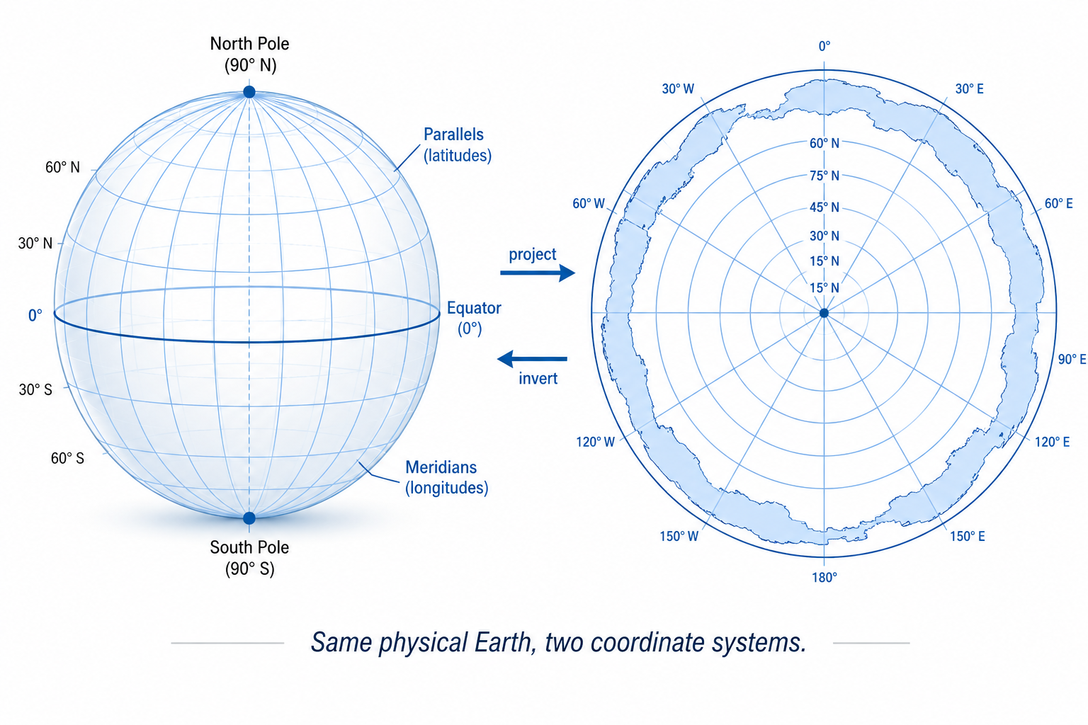
This map sends the North Pole to the center of the disk, the equator to the middle circle of the disk, and the South Pole to the outer boundary.
There is an important technical qualification here. Away from the South Pole, this map is smooth and one-to-one. The sphere with the South Pole removed corresponds to the open disk of radius πR. At the boundary, however, the South Pole is represented by an entire outer circle. That means the closed disk is not literally a one-to-one copy of the sphere unless we identify the whole outer boundary as a single point.
So the precise statement is this:
The open disk is a smooth coordinate chart for the sphere with the South Pole removed. The full closed disk represents the full sphere when the entire outer boundary is collapsed or identified as one point.
This is why the “ice ring” language can be useful symbolically, but must be handled carefully mathematically. In Claim A, the outer boundary is not a normal Euclidean edge of the world. It is the projected representation of one polar point.
The Metric Is the Load-Bearing Fact
The sphere’s intrinsic metric is:
ds² = R² dφ² + R² cos²(φ) dθ²
Substitute r = R(π/2 − φ). Then dφ = −dr/R, and cos(φ) = sin(r/R). The metric on the disk becomes:
ds² = dr² + R² sin²(r/R) dψ²
This is not the Euclidean flat metric of the page. The ordinary Euclidean polar metric would be:
ds² = dr² + r² dψ²
Those are different metrics. Near the center they approximately agree, because sin(r/R) ≈ r/R when r is small. But as r approaches the outer boundary, the difference becomes decisive. At the equator, where r = πR/2, the circumference factor in the spherical metric is R, while the Euclidean disk would use πR/2. The ratio is 2/π ≈ 0.637. That is a major discrepancy, not a rounding error.
This is the load-bearing fact of the whole argument:
The disk that reproduces sphere observations is not metrically flat. It is the sphere drawn in azimuthal coordinates, with the curvature carried by the metric.
For a less technical reader, a metric simply means the rule for measuring. If you put a ruler on a normal sheet of paper, you are using the paper’s Euclidean metric. But a map does not have to use the paper’s measuring rule. A subway map, for example, can show order and connection without showing true physical distance. A globe map projected onto a disk can also have a measuring rule that says, “Do not measure this by the flat page. Measure it by the sphere that this disk is representing.”
So the disk may look flat to the eye, but its measurements are not flat-paper measurements. The hidden rule of measurement is spherical. That is why the disk can preserve the same distances and paths as the sphere when handled correctly.
Why “Metric Equivalence” Is the Right Term
The earlier title used the phrase conformal equivalence. That was not the best mathematical wording. A conformal map preserves angles. The azimuthal equidistant projection is not generally conformal. It preserves distances from the center and directions from the center, but it does not preserve all angles everywhere on the disk.
The stronger and more precise claim here is not conformal equivalence. It is metric equivalence after the disk is equipped with the pulled-back spherical metric.
In plain language: the disk and sphere give the same geometric measurements because the disk is carrying the sphere’s metric. The disk is not pretending that the flat page’s ruler-distance is real distance. It is using a different measurement rule, and that measurement rule is exactly the spherical one rewritten in disk coordinates.
Why This Is Sufficient for Claim A
The reason this construction proves Claim A is a standard principle of differential geometry: when a smooth coordinate transformation carries the metric correctly, intrinsic geometric measurements are unchanged. Distances, angles, areas, geodesics, local curvature, and parallel transport can be computed in either coordinate system and give the same numerical result.
Stated plainly: if the disk carries the spherical metric, then the disk and the sphere are not two different intrinsic geometries. They are the same intrinsic geometry described with different coordinates.
There is another important qualification. Some observations are purely intrinsic to Earth’s surface: surface distances, shortest paths, local angles, latitude/longitude relationships, geodesics, and many navigational computations. These are directly covered by the surface metric.
Other observations involve the surrounding three-dimensional physical setup: eclipse shadows, satellites, light paths, elevations above the surface, and celestial viewing geometry. Those remain identical only when the whole physical configuration is transformed consistently along with the surface. That is not a weakness of Claim A. It is the correct way to state it. A coordinate transformation must transform the whole model, not only the ground beneath the observer.
Claim A proves equivalence when the disk, the metric, the observer, the heavens, and the measurement process are all treated as the same physical model written in different coordinates.
Observation 1: Surface Distance and Flight Paths
Take two cities in the southern hemisphere: Sydney and Santiago. On a Euclidean flat-earth map, these places appear extremely far apart, and the straight-line page distance can become wildly inconsistent with actual flight times.
But Claim A does not use the Euclidean page metric. It uses:
ds² = dr² + R² sin²(r/R) dψ²
With that metric, the shortest path on the disk is the same path as the great-circle route on the sphere, only drawn differently. The path may look curved on the disk, but the metric makes that curved-looking route the true geodesic. The numerical distance is unchanged because the disk is only a coordinate representation of the sphere.
This is one of the clearest ways to distinguish Claim A from Claim B. Claim A survives ordinary navigation because it is using the same geometry as the sphere. Claim B, if it insists on ordinary Euclidean ruler-distance across the disk, must supply additional physics to explain why distance, speed, and travel time still come out as observed.
Observation 2: The Horizon
On the sphere, the visible horizon depends on Earth’s radius and the observer’s height above the surface. At ordinary human height, the horizon is only a few miles away. As the observer rises, the visible distance grows according to the familiar curved-surface relationship.
On the disk with the projected spherical metric, the local surface geometry is the same. If the observer’s height and line of sight are included as part of the transformed physical setup, the horizon calculation gives the same result. The disk does not avoid curvature here. Rather, the curvature is built into the metric.
So Claim A does not say, “A Euclidean flat disk naturally gives the spherical horizon.” It says something more precise:
The projected disk gives the spherical horizon because it is the spherical geometry expressed in disk coordinates.
Observation 3: The Two Celestial Poles
On the sphere, Earth’s rotation axis defines two poles. Observers in the northern hemisphere see stars rotate around the north celestial pole. Observers in the southern hemisphere see stars rotate around the south celestial pole. This is one of the most important observational tests because the sky does not behave as though there is only one visible center of rotation for every observer on Earth.
In Claim A, the two-pole structure is preserved. The North Pole maps to the center of the disk. The South Pole maps to the identified outer boundary. The celestial sphere and its axis must be transformed with the same coordinate logic as the Earth’s surface. When that is done, the same sky observations are recovered in disk coordinates.
This again shows the difference between a projected disk and an ordinary Euclidean disk. A Euclidean disk with a simple dome above it has to explain why southern observers see a distinct southern celestial pole. A projected disk carrying the spherical model already contains that structure, because it has not changed the underlying geometry. It has changed the coordinate vocabulary.
Observation 4: Lunar Eclipse Shadows
A lunar eclipse is not merely a two-dimensional surface-distance problem. It is a three-dimensional geometry problem involving the Earth, Sun, Moon, and light paths.
On the ordinary sphere model, Earth’s shadow on the Moon appears with a circular edge because Earth is a sphere in three-dimensional space.
Claim A preserves this result only if the surrounding three-dimensional configuration is also treated as the same physical model expressed in transformed coordinates. The disk drawing by itself does not become a Euclidean plate casting a plate-shadow. Under Claim A, the “disk” is not a new solid object replacing the sphere. It is the sphere represented in azimuthal coordinates. Therefore the eclipse geometry is the same because the physical object and the light geometry have not been changed.
This distinction matters. Claim A should not be used to say, “A literal Euclidean disk casts the same shadow as a sphere.” That would be Claim B, and it would require new physics. Claim A says: “The sphere represented as a metric disk gives the same eclipse result because it is still the same geometry.”
Observation 5: GPS and Satellite Geometry
GPS is also not merely a surface-distance calculation. It depends on satellite positions, signal timing, clocks, relativity corrections, and an Earth reference model.
Within Claim A, GPS works on the disk for the same reason it works on the sphere: the disk version is not a different physical world. It is the same coordinate system rewritten. If satellite positions, receiver positions, clocks, and signal paths are all transformed consistently, the same receiver fix results.
But this should be stated carefully. The surface metric alone does not magically reproduce every satellite observation. The full physical model must be carried over. When it is carried over, the results are identical because a coordinate transformation does not change the underlying physical relationships.
That is the precise claim. It is also enough.
The General Theorem, Stated Carefully
The proof of Claim A can now be stated formally:
Let M and N be smooth Riemannian manifolds away from the projection singularity, and let Φ: M → N be a smooth coordinate transformation that carries the metric of M to the metric of N. Then every intrinsic geometric measurement on M has an exact counterpart on N giving the same numerical value.
Applied here, M is the sphere with the South Pole removed, N is the open azimuthal disk, and Φ is the azimuthal projection. The boundary of the closed disk represents the missing South Pole only after the whole boundary is identified as one point.
With that qualification in place, the conclusion follows:
The sphere and the projected disk with the pulled-back spherical metric are the same intrinsic geometry in different coordinates.
This is not a claim that the ordinary Euclidean disk is empirically equivalent to the sphere. It is a claim that the metric disk and the sphere are one mathematical object described in two ways.
The Theological Connection: Plan, Pattern, and Embodiment
For those working within a firmament cosmology, this result is not a defeat. It is a synthesis.
Scripture often speaks in ordered, plan-view language: the face of the earth, the circle of the earth, the four corners, the ends of the earth, the foundations, the boundaries of the sea, the circuits of the lights, and the appointed times. That language can sound flat because it is describing the world as an ordered domain under heaven — a world with center, boundary, direction, measure, and covenantal purpose.
But a plan-view description does not have to cancel a dimensional form. A builder can begin with a flat drawing and then raise the building into depth. The drawing is not the whole building, but the building is not disconnected from the drawing. The drawing gives the order; the building gives the embodiment.
That may be the most helpful way for ordinary readers to understand Claim A. The disk can be read as the blueprint or plan-view of the created order. The sphere can be read as the same order expressed in physical dimensional measurement. The two are not automatically enemies. They may be two levels of description: the written plan and the built form.
In this framework, the firmament language can be read as a coordinate vocabulary for the heavens as seen from within creation. The “circuits” of the heavenly bodies, the heavens stretched out like a tent, the world ordered around signs and seasons — these are not automatically refuted by the mathematical fact that the Earth’s surface geometry is spherical. They may be describing the same ordered creation from another vantage point.
The “ice wall” at the edge of the disk must therefore be handled with care. Under Claim A, it is not a normal outer edge in Euclidean space. It is the South Pole/Antarctic region represented by the boundary behavior of the projection. If the entire boundary is identified as one polar region, the disk representation closes back into the sphere.
So the disk language can preserve the meaning of circle, boundary, center, and circuit without requiring us to pretend that ordinary flat-paper distances are the true distances on Earth. The disk is not merely a drawing. It is a way of writing the sphere from the perspective of ordered surface, appointed motion, and covenantal place.
“It is he that sitteth upon the circle of the earth, and the inhabitants thereof are as grasshoppers; that stretcheth out the heavens as a curtain, and spreadeth them out as a tent to dwell in.”
Isaiah 40:22
The same heavens. The same earth. Different language for describing what God built.
What We Have Proven
To restate clearly: Claim A is the proposition that the flat-disk representation of Earth, equipped with the azimuthal-projected spherical metric, is mathematically equivalent to the standard spherical surface geometry. Surface distances, geodesics, angles, local geometry, and navigational relationships produce the same numerical results.
For observations involving surrounding space — eclipses, satellites, heights, light paths, and celestial viewing — the equivalence holds when the entire physical configuration is transformed consistently, not when only the ground map is redrawn while everything else is left as a naive Euclidean picture.
Within Claim A, there is no empirical evidence that can distinguish the sphere from the metric disk, because there is no different physical geometry to detect. The choice is a choice of coordinates and vocabulary.
That is the value of Claim A. It lets the disk language be made mathematically rigorous without pretending that the Euclidean page metric is the true metric of Earth.
In Plain Terms
Here is the whole argument in ordinary language:
- A normal flat map lies about distance because it uses flat-paper measurement.
- A projected disk does not have to use flat-paper measurement.
- If the disk uses the sphere’s measuring rule, then it gives the same results as the sphere.
- That means the disk can be a true coordinate description of the sphere, not a rival physical object.
- The flat language may therefore function like a blueprint, pattern, or covenantal map, while the sphere is the same order expressed in built-out dimensional form.
This is why Claim A matters. It gives ordinary readers a way to understand why biblical or symbolic flat-earth language does not have to collapse the moment spherical measurements are introduced. The language may be operating at the level of plan, pattern, and ordered domain, while the physical measurements operate at the level of embodied geometry.
Flat as blueprint can coexist with spherical as embodiment. Flat as ordinary Euclidean physics is a separate and much harder claim.
Where Claim B Becomes Necessary
What Claim A does not prove — and deliberately does not prove — is that the disk is geometrically distinct from the sphere.
The disk in Claim A has the projected spherical metric. That means it is not a different surface geometry. It is the sphere in azimuthal coordinates.
For someone who wants the disk to be a metrically distinct reality — flat in the literal Euclidean sense, with ruler-on-page distances corresponding to physical distances on Earth’s surface — Claim A is not enough. That requires Claim B: the proposition that a Euclidean-flat disk can be made consistent with observation through additional physics, such as refractive media, distance-distorting fields, nonstandard optics, or other structures within the firmament.
Claim B is a much harder mathematical and physical exercise. It cannot rely on coordinate transformation alone, because coordinate transformation does not create a new geometry. It must produce new physical rules and then show that those rules match observation without ad hoc patching.
For now, Claim A stands in its corrected form:
The disk and the sphere, in their mathematically rigorous forms, describe the same Earth only when the disk carries the projected spherical metric. The disk is not Euclidean-flat; it is the sphere written in disk coordinates.
Claim A, Made Operational
The argument above is best handled, not just read. Two companion apps render Claim A directly — the same observer, the same stars, the same horizon, drawn first as a sphere and then as a disk. Drag the figure in either app and the visible hemisphere changes; flip between the two and the picture changes while the data underneath stays identical.
- The Witness Disk — The same cosmos in azimuthal projection. The North Pole is at the center, the equator is the circle halfway to the edge, and the South Pole is represented by the identified outer boundary.
- The Three Witnesses — Drag a figure around the globe and the horizon sweeps the celestial sphere. The two polar witnesses fix the axis; the same data is shown in sphere coordinates.
The apps are cross-linked at the top so you can toggle between projections with a tap. The math underneath is the projected metric ds² = dr² + R² sin²(r/R)dψ² — the equivalence this essay proves, walked through by hand.